MCC GIS Summer Internship
Documenting our time in Orono at the University of Maine while doing research in collaboration with CAFS at Wheatland Geospatial Lab.
Documenting our time in Orono at the University of Maine while doing research in collaboration with CAFS at Wheatland Geospatial Lab.
Funding provided by Skills Training in Advanced Research & Technology (START) Supplemental Funding Request for ATE at Monroe Community College (Award #1955256) with IUCRC Phase 3 at University of Maine - Center for Advanced Forestry Systems (CAFS). Available for educational use only. Created Summer 2022.
Bryan and I were lucky enough to be selected for the MCC GIS summer internship that finds MCC partnering with the Center for Advanced Forestry Systems (CAFS), located at the University of Maine campus in Orono. We will be working alongside research team at the Wheatland Geospatial Lab to help document, identify, and classify tree species within the state of Maine using geosptial and AI machine-learning prediction tools to complete this task.
We started our journey in the early hours on Monday, June 13. Flying from Rochester to Bangor via Newark, we arrived at our destination before noon where we were picked up by our professor Jon Little, who immediately suggested we visit Stephen King's house.
Several people were already outside taking pictures when arrived. Sadly, Mr. King was not home.
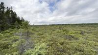
We got lunch and drove to the campus to get settled into our dorms. Excited to see our new surroundings, we headed to the Orono Bog Boardwalk.
The Orono bog was formed in a similar manner.
The Orono bog is the reclamation of a lake with wetland plants. It started out as a basin with a lake and non-wetland plants growing harmoniously, until the basin became waterlogged, suffocating the non-wetland species and causing them to sink and decompose at the bottom of the lake, while allowing for the rapid spread of wetland plants to grow within the basin and completely cover the lake surface with peat, the decomposing byproduct of plant matter. While it may look like solid ground, the peat is completely saturated with water, creating a sponge-like surface that squishes when compressed. Some parts of the bog have peat beds that are over 20 feet deep.
(LEFT): Bryon reading about the different plant species in the bog. (RIGHT): Jon looking over the edge of the boardwalk. The treeline in the back delineates the bog's edge. The dead conifers on the left show where the bog edge was in the past, but has since become waterlogged and suffocated the trees. The surrounding wetland plants feed off of the nutrients and are seen thriving across the majority of the bog's surface.
Panoramic video by Casmir showing the sheer size of the bog. This peaty surface is over 20 feet deep in some areas.
Day 2 saw us finally exploring the Barbara Wheatland Geospatial Lab where we'd be doing most of our research. Located in Nutting Hall, we were introduced to researchers Dan, Tony, and Dave. They will be mentoring us and overseeing our projects.
After a tour facility, we went into town for lunch with Jon at Tacorita, and then obtained fishing gear and licenses. We walked down to the Stillwater River next to our dorms and attempted to see if any fish were biting. Unfortuantely for us, there were only mosquitoes and blackflies.
We found a greenhouse adjacent to the Wheatland lab, where there was a massive American agave plant was growing, along with others such as banana trees and succulents.
Tony giving a presentation on remote sensing and data collection/processing.
By Day 3 we were given an overview of one of the research projects we would be working on this summer. We met with Assistant Research Professor Kasey Legaard, who explained his project: attempting to calculate the biomass of individual trees in a forest using only satellite imagery. He explained how he has written 20 to 30,000 lines of code in his script, but that isn't the most tedious part: in order for the script to run accurately, it needs to be have cloud-free imagery to process. Therefore, we will be maually creating training points to identify clouds in raster images, pixel by pixel. These points will then be run through the Random Forest machine-learning software alongside cloud-free images, and we will compare the results to see how well the AI can automate the masking of clouds in multiple images, compared to other methods that Kasey has previously tried.
After lunch with the Wheatland team, Tony gave us an overview of LiDAR and how data is collected for the school, which uses its own Cessna plane. We were also briefed on the field work we'd be doing with research assistants Stephanie and Rissa next week in the Penobscot Experimental Forest.
Kasey explaining the process of cloud masking to Casmir.
Our morning began with Kasey having us do cloud masking on our own. We labeled pixels as either O (cloud), C (clear), or S (cloud shadow). The machine-learning process requires multiple examples as input to have an accurate AI output, so the manual pixel classification is extremely time-consuming. Kasey even explained how he convinced his daughter it was a game to try and get her to help him out.
We also had a workshop with Tony and Dave, where we worked with LiDAR data to produce 3D maps and predictions using R Studio.
Portion of the R code written and one of the final products shown on the right, a 3D image created with LiDAR return points.
Easy 1-mile loop extends over the bog with picturesque views. Read more about the history here.
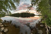
Shallow spot with crystal clear water. Great for viewing the sunset and right across the street from our dorms!
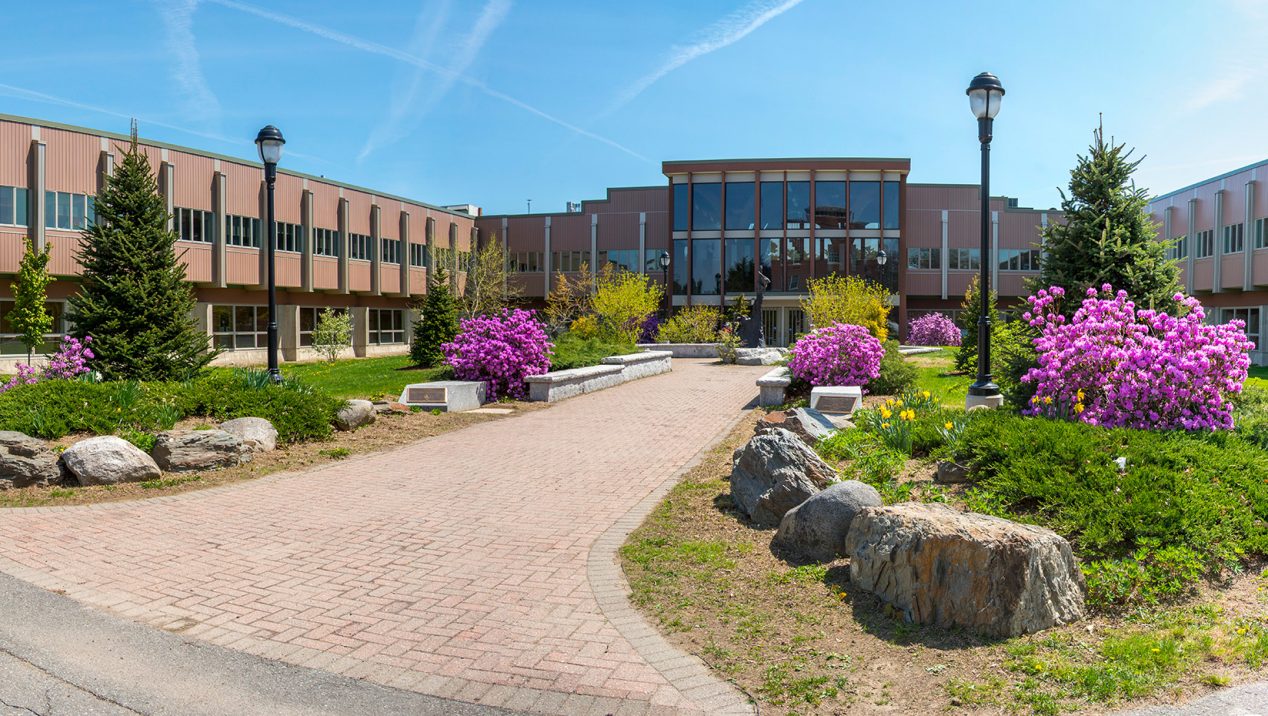
Contains the Wheatland Geospatial Lab and research offices for CAFS.
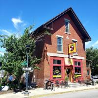
Ate a great lunch here in town. Check out their menu!

Picked up bug spray and tick repellent for when we do field work. Main focus is rock climbing and hiking gear.
Picked up fishing gear and licenses.
Easy 1-mile loop extends over the bog with picturesque views. Read more about the history here .
Shallow spot with crystal clear water. Great for viewing the sunset and right across the street from our dorms!
Contains the Wheatland Geospatial Lab and research offices for CAFS .
Ate a great lunch here in town. Check out their menu !
Picked up bug spray and tick repellent for when we do field work. Main focus is rock climbing and hiking gear.
Bryon waiting for the bus to return our bikes to Bangor.
We had the day off due to Juneteenth.
This past weekend, we rented bikes from Ski Racks Sports in Bangor. Bryon and I had to return them today, so we embarked on a 4.5 hour public bus ride (there's a driver shortage!) to the city. By the time we returend to Orono, the forestry field work team of Steph, Rissa, and Dave had just finished for the day, and picked us up to celebrate Casmir's 30th birthday at Mason's Brewery.
Bryon's catch of the day, a small mouth bass!
We were scheduled to meet with Kasey this morning, however his family came down with a nasty cold, so cloud masking was postponed.
Instead, we worked with Tony and Dave to test run the LiDAR workshop one more time, before having us install the data to each workstation in the Wheatland Geospatial Lab. Today was a light day and we were finished by noon, so Bryon and I went down to the river to see if any fish were biting. Bryon managed to snag 2 small mouth bass. We decided to go to bed early since we had a long day ahead of us.
Locations for all 7 plots visited to collect research data. While seemingly close, the lack of bridges over the Penobscot River paired with 25mph speed limits turns a 4.4 mile distance into a 30 minute drive.
First two days of field work! Steph and Rissa picked us up at 7am to head over to the Penobscot Experimental Forest. We would be locating Continous Forest Inventory (CFI) plots. These plots have been established by the US Forest Service (USFS), and they seek to determine growth by repeated invetories of permanent plot samples. The plots that we visited had been monitored for at least 40 years, and it was our job to collect data on the current landscape.
The general workflow is below:
Plot locations were given as GPS coordinates, so we hiked to the general area. Once there, we had to dig through the leaves on the forest floor to find a knitting needle marking the official CFI plot center.
In the photo to the left, we've found the knitting needle of a plot with the help of a blue tape attached to its head. We will then begin setting up the trimble upon this location. The trimble is used to aid in precise surveying and measurement. For this study, we calibrated the device with 500 satellites.
Stephanie teaches Wayne how to use the trimble. While calibrating, the trimble must not be disturbed. This process may take some time depending on how many satellites are chosen to calibrate with.
Once calibrated, we marked the center plot with a pin of our own as to not disturb the CFI needle. It also had a hoop that we attached logger's tape to it, and measured out points of 5.75m and 10m radii in the cardinal directions. We would be identifying all trees within these areas that had a diameter breast height (DBH) of 10.2 inches or wider. The 5.75m markers denoted a square plot, while the 10m markers marked a circular plot. The square plot is part of a separate study done by Rissa to compare the differences in plot shapes. For example, a tree could have been 5.75m on a cardinal direction and could be counted for the square plot, but a tree 5.75m on a NE direction would not; therefore, more precision was needed to define which trees fell within the square plot.
From left to right: The center pin of the plot. Rissa and Casmir denote plot boundaries. Wayne uses the Haglöf distance measuring device to see how far away he is from plot center.
After defining the plots, we began to identify all trees within it that met the DBH criteria. This required two teams: one to remain at plot center, and one to seek out the trees.
The tree-seeking team duties are as follows:
A Haglöf device (right) and its transponder (left).
(LEFT): Bryon measuring tree distance from plot center. (CENTER): Wayne collecting DBH data. (RIGHT): Tree has already been marked with a CFI ID number.
The stationary team duties are as follows:
(LEFT): Casmir & Rissa recording data. (CENTER): Wayne calculating azimuth with a compass. (RIGHT): Casmir using a BAF prism to identify variable point samples.
Wayne calculating the distance to the base of the tree with the Haglöf device.
After all qualifying trees had been identified and classified, samples were selected for each unique DBH value. The tree-seeking team the attached the Haglöf transponder to the tree at breast height, while the stationary team uses the Haglöf device to calculate a tree height estimate. We ran into a few problems where we forgot to mark the trees, which sometimes made for a cumbersome search.
A clinometer used to calculate tree height angles.
Because the Haglöf operates with ultrasound, sometimes natural disturbances, such as wind, or human interference can result in erroneous values. Instead, a clinometer can be used to manually calculate the tree height with the pythagorean theorem.
Tree height = (base angle / crown angle) * distance from base
(LEFT): Diagram showing all points used to calculate the tree height. (RIGHT): Casmir using the Haglöf device to automatially calculate tree height.
There were pros and cons to boths days out in the forest. On day one, we encountered a lot of interference, and extremely dense vegetation, rendering the Haglöf useless. Therefore, we had to use the clinometer to calculate all heights, and weave loggers tape through the branches to set our boundary distances. The process of finding the crown height was extremely difficult, especially in more dense vegetation where all trees started to blend together. We were able to get more work done on the first day, but the second day saw Bryon and I leading the team and showing off what we had learned. While it was exciting to get more hands-on experience, our plot locations were located in a bog. The temperature was much warmer, and the air moved far less. One misstep and you could be knee deep in peatmoss. The silver lining to the challenging landscape was far fewer trees located in the bog than other plot sites, and we could now use the Haglöf to quickly calculate our distances.
With Kasey still out of work tending to his family, we had another light day. We ended up Zooming with Wayne, and decided to take it easy as we prepare to head off to Fort Kent on Monday.


Our itinerary for Monday. We left from Orono and made a pit stop near Mount Katahdin before arriving at Fort Kent.
The underwhelming view of Mt. Katahdin during the rainstorm.
Today we traveled four hours northward to Fort Kent. On our way up we tried to stop at a scenic viewing spot to see Mount Katahdin, but our hopes were dashed due to the gloomy and wet weather. We were nervous that the rain may impact our schedules, but by the time we arrived at Fort Kent, the rain had stopped!
Our first stop here was Cyr Hall, where Ned Rubert-Nason gave us a warm welcome. He is the a leader of the forest management team, and gave us a quick overview of some of the equipment we would use the following day.
Dusk at The Lodge dorms in Fort Kent. Some lingering rain clouds spent the night, but were gone by early morning.
We planned our itineary for the week, where would be working with three different teams. Tuesday and Thursday would see us working with Ned's team from Fort Kent studying the tree morphology from the ground, along with Peter from the Schoodic Institute flying drones above the trees; Wednesday would be our day with Nicole and Jasmine's team, studying tree regeneration in various types of drainage basins.
Evening was approaching quickly, so we settled into our room at The Lodge dorms. Paradis Supermarket was convienietly across the street, and we stocked up on groceries for the week. It would be an early night for us, as we had our first day of field work with a new team at 7:30 am the next morning.

Locations of all field work sites for our week. It took about an hour to get to the Hewes Brook Road sites, and we met up with the various teams at Coffin's General Store in Portage Lake. Coffin's proved to be an oasis on the border of the forest, where the nearest flushable toilet could be found for miles.
Our day started promptly at 7:30am, with Bryon, Casmir, and Wayne meeting Ned at Cyr Hall. We were introduced to Taylor, Jonnie, and Saja -- our teammates for the day. We set off southbound towards Portage Lake, where we would meet up with Peter and his apprentice, Peter B at Coffin's General Store. After some delicious breakfast sandwiches, we headed towards our first of four sites located off a logging road in the Northern Maine Woods.
Just off the road was a large clearing where we would start. After a detailed briefing on the instruments we'd be using by Peter, the team was split into smaller groups to work on various projects.
Taylor and Saja began identifying trees of interest (red & white spruces, balsam poplars) and labeling them.
Bryon, Casmir, and Peter B started with the leaf spectrometer on all unique species.
Peter, Ned, and Wayne began setting up the drone for its flight, and Jonnie began using the LIcor machine to measure the uptake of CO 2 and release of water vapor from plant samples.
Jonnie, Taylor, and Saja stayed behind at Site 1 to continue to label trees and collect LIcor samples, while everyone else proceeded to the Site 2.
Here, Ned began to mark trees that would need their morphology studied in the following two days.
Peter B and Casmir collected leaf data with the spectrometer, while Bryon got to work more closely with Peter and the drones.
Venturing deep into the clearing, Ned, Peter B, Bryon, and Casmir continued marking trees and collecting spectral signatures of leaves. We didn't want to venture anywhere that the drone could not see, so only the perimeter of the clearing had collectable data. Even with the open field, some of the trees were still hard to access, as the rainstorm thhe day prior had created muddy puddles hidden by the overgrowth.
Peter and Wayne collected more drone data, however this site had previously been photographed within the past year, so a smaller area was chosen. The clouds were a nuisance, but the drone team managed to catch pockets of sunshine that allowed for the clearest imagery.
The tree morphology team finished before the drone team, and got a chance to watch another successful drone landing.
The final site was the quickest, due to the leaf spectrometer running out of battery power. Instead, a handful of trees were marked for further study by Ned, while the rest of the team observed the drones. This area had been photographed just before spring, unlike the other sites; therefore, a tighter flight pass was required, but this was accomplished in record time as the sun was now fully shining with little to no clouds in sight.
After a day of hard work, we headed back to Fort Kent to start processing the drone data.
The two drones used to capture aerial imagery, the DJI Phantom 4 (left) and the DJI Matrice 600 (right).
We used two different drones to collect data during the day. We used a smaller DJI Phantom 4 drone to fly over and collect just the RGB images, and a larger DJI Matrice to do scans with a larger range of wavelengths collected by a much more sensitive sensor.
Peter engaging the drone for take-off.
Both drones flew pre-programmed flight paths so as to cover the entire area that needed to be scanned with enough image overlap to line it all up. To program the flight, the Matrice was plugged into a laptop computer and the path was loaded into the drone. Once uploaded, the cord was disconnected and the flight began. Take-off was done manually by Peter and once the drone got to its programmed starting point, the program took over and the drone flew its automated flight path before returning to the end point, where Peter regained control for landing. The drone was then plugged back in, and the data from the sensor was transferred to the laptop. The same process occurred with the Phantom, with the only exception being that the Phantom did not have to be plugged in to recieve the path information or to transfer the collected data back. Over 47 GB of imagery was collected during the day.
The visible light spectrum, with colors occupying different nanometer wavelengths.
Spectroscopy is a technique that measures the different spectra of light that are absorbed or reflected by any matter. Based off of the wavelengths of light reflected, the signature can be used to determine factors of plant health. Changes in the spectral signature could be due to differences in the NPK levels.
The trigger portion of the spectrometer. We used a slightly different model, but the process is the same.
To gather the spectral signatures of leaves, we used a specialized portable leaf spectrometer. A lithium-ion battery that had to be kept cooled was worn in a backpack, while a handheld trigger device was connected with a fiber optic cable that could read the leaf signatures. Once the trigger was pulled, the signature appeared on a wireless tablet. The signatures collected would be compared them to healthy signatures to see which plant samples were stressed or unhealthy.
Below on the left is an example of spectral signatures of different land types. Water has a very low signature, as it absorbs the most light. The sharp uptick in the green vegetation signature between the visible and NIR wavelengths is called the "red edge", where wavelengths before it are absorbed by chlorophyll, and the spike afterwards is indicative of different values of NPK biochemical markers, while the dip following the spike is due to plant water absorption. On the right side image is an example showing the difference in spectral signatures of healthy and unhealthy vegetation. The dry vegetation has a lower green reflectance and less water absorption.
(LEFT and CENTER): Peter demonstrating the leaf spectrometer to the team. The large lithium-ion battery is seen in left corner of the yellow device. It took about 15 minutes to warm up before use, and came with four replacement batteries which we used up completely. (RIGHT): Bryon wearing the spectrometer backpack, while Casmir uses the wireless tablet to label and view each sample's spectral signature.
(LEFT): Collecting data from Hewes Brook Road Site 3. Ned can be seen in the background (in orange) labeling trees for Peter B and Casmir to further study with the leaf spectrometer. (RIGHT): The Matrice drone flying above the site. It's the tiny little black speck amongst the lower left cloud.
Jonnie was in charge of using the LIcor machine to further analyze plant samples. According to Licor.com , the LI-6800 is designed to non-destructively probe processes involved in photosynthesis. First, the LI-6800 measures uptake of carbon dioxide (CO 2 ) and release of water vapor (H 2 O) by a sample with high precision infrared gas analyzers (IRGAs). For leaf-level measurements, additional measured parameters, including leaf temperature, allow the instrument to calculate other physiological parameters, including stomatal conductance (g sw ) and intercellular CO 2 concentration (C i ). Second, the LI-6800 quantifies fluorescence yield (Φ F ). Fluorescence yield provides information about the light reactions of photosynthesis.
This was a time consuming process, and not all of the samples collected could be processed the same day.
Bryon managed to find a snake at one of the sites, along with several butterflies and moths. To remind us that we were in the true wilderness, we also found remnants of a predator's dinner.
Today Bryon and Casmir split up from Wayne, and went with Nicole and Jasmine to gather data for their weather sensor project, while Wayne met up with Dave Sandilands in Ashland to gather drone data from the sawmill.
Wayne and Dave working at the sawmill to collect drone imagery.
We would be working with Professor Nicole Rodgers, and her Masters student, Jasmine. For Jasmine's project, she would be studying the difference in tree regeneration in various plots with different soil drainage types.
The first plot was located in a poorly-drained site. Nicole set up the weather sensors that would be placed at each station, while Casmir, Bryon, and Jasmine began to classify the trees within the plot and count the number of new sprouts.
The next plot was a fairly-poor drainage basin. Pictured above is one of the weather stations installed. These will be periodically monitored several times over the next two years, collecting data on temperature, wind, and humidity. These were installed 1 meter away from the CFI plot marker.
Continuing uphill, site 3 was a moderately-well drained plot. The more well drained the soils were, more regerative growth was found.
The fourth site was on a steep slope, allowing for well-drained soils. This resulted in the most new sprouts found, which numbered over 100 within a 3.5ft radius plot. We unfortunately ran out of pipe cleaners to mark each new bud, which cut our day short.
First, we identified where the CFI plot was, and then installed the weather sensor 1 meter from its point. Using the center of the CFI plot, a 15 foot radius was established at each cardinal direction. From these points, North, Southwest, and South East were selected, and an 3.5 ft radius was established around these points. Within the 3.5ft radii, it was broken up into 4 quadrants to easily sort the data collection, and all new regenerative tree growth was identifed by species and height class.
Site Classification:
Site 3, a moderately drained soil plot. You can see how the regrowth is affected by the lack of growth in two of the quadrants, but much heavier in the other two.
The first two plots had far less regenerative growth within the plots, which made them quick and somewhat easy. The biggest challenge were the mosquitoes, as the moist enviroments allowed them to thrive and be more of a nuisance than the moderately and well-drained sites.
Site 4, the well-drained plot with the most regrowth. New buds tended to be either sugar maple, or moose maple.
The final two plots were located on somewhat steep hills, which made the field work a lot more difficult. It was hard to keep the measuring sticks in place, and these sites also had far more regenerative growth. Keeping track of the counted buds was extremely difficult, as many of the species were the same and clustered together.
The team noted how much faster it was with two extra sets of hands to count and mark the plots, as they had spent the previous day with only two teammates that spent over 2 hours on a single plot with over 200 new buds.
Close up of the regenerative buds marked with pipe cleaners. These will remain on the buds until the next check-in in a couple of months. They will be monitored several times over the next two years to study their growth rate and the impact of the drainage type on the amount of regrowth. We unfortunately ran out of pipe cleaners and were not able to get to a prospective 5th location.
Since we finished early, Bryon had the rest of the day to explore the town of Fort Kent in search for new fishing spots. He visited the Blockhouse Fort, which is the only fortification relating to the "Bloodless" Aroostook War of 1838-1839, and the border dispute between Great Britain and the United States. Read more about the fort here .
Bryon
Sites 1 -3 on Hewes Brook Road. Some of the sites were areas that had been salvage clearcut within the past few months.
Bryon
Casmir happened to have his friend, Amanda, in the state for the July 4th weekend. He went to her family's campsite about an hour away near Jo Mary Lake, where there were some amazing views of Mount Katahdin during sunset on a kayak ride, where he went swimming with her family in the lake afterwards.
Happy Independence Day! No work scheduled.
At 9:30am we met up with Kasey to reevaluate our progress with the cloud masking. As he had dealt with his family falling ill the week before we left for Fort Kent, we hadn't gotten as far with the project as we had hoped. Kasey would spend the rest of the day feeding our training samples into the machine-learning algorithm to produce AI output of cloud masks. We would be able to work with the data on Wednesday, and have another go at training samples.
Kasey, Casmir, and Bryon working on Round 2 of training samples for cloud masking.
At 10am, the team met with Tawanda Gara, a remote-sensing postdoctoral research associate at Nutting Hall, who gave us an overview of his research project to study biochemical properties of trees within the forest with satellite imagery.
The goal of his study is to find a possible way to identify plant stress with biochemical indicators from remote sensing imagery before any of the physical effects can be seen, in order to preventatively protect vulnerable tree populations. He explained his workflow for processing leaf samples:
With the leaf scans, the Leaf Area Index (LAI) can be calculated to estimate the amount of leaf material within the canopy. This number has no units, as it is a ratio of leaf area to ground areas. This number can determine whether a tree canopy is healthy or stressed.
After the samples have been processed, the hyperspectral signatures of each were compared to spectral signatures of healthy/normal tree species. This will show exactly where there are discrepancies, indicative of unhealthy trees or plant stress.
These signatures were also fed into machine-learning models, which contained multiple spectral libraries that could allow the reflectance per leaf to estimate the condition of the entire tree. Matlab and Random Forest software was usd to run the packages, studying four prospective traits: Tree Height, Leaf Area Index, chlorophyll, and NPK.
Since the imagery from DESIS that he used for the project is not open source, he had 235 spectral bands to work with, compared to Landsat or Sentinel imagery's 11 or 13 bands. He would be utilizing parametric (DESIS hyperspectral) and non-parametric traits (PSLR regression, Random Forest regression, VSURF variable selection, and MNF bands to simplify the model, as he noticed that he could gather accurate information from a selection of the 235 bands.
Depending on the band combination, different traits were highlighted. For the nitrogen band combo, spikes near the red edge stood out at the 700-990nm signature, and the models predicted a regression of .75. For the chlorophyll canopy band combo, the visible light range of 557-621nm were utilized, and predicted a regression of -.66.
Overall, Tawanda is looking to assess the spatial consistency between parametric and on-parametric data.
After meeting with Tawanda, we were introduced to PhD student Rajeev. He spent the next hour explaining to us the similarities and differences between remote sensing and GIS, and how they relate to one another. He also explained the pros and cons of working with only one software versus a range of softwares. Random Forest is the best and most efficient for working with large amounts of data. If he were to use ArcGIS Pro to accomplish the same task, he would have to process each raster individually, rather than as a set. This can also be accomplished with Python coding, but his experience with Python is less than that of R-code. Within Random Forest, he is able to utilize raster and RGDAL packages to combine bands.
Wayne finally got to meet Tony and Dave from the Wheatland Lab today, although it is also his last day here with us before heading back to Rochester.
Dave had processed the drone imagery taken from last Wednesday in Ashland. He displayed the data for us in Agisoft, a software that digitally processes photgrammetric imagery and generates 3D spatial maps. He offered us a chance to take more photos next week in a small test forest located on the Orono campus. We're really looking forward to collecting our own drone data and seeing how it will be mapped!
Tony gave an overview of the Wheatland Lab and its current projects and goals to Wayne (Bryon and Casmir viewed this presentation during the first week).
Afterwards, we finalized our schedule for the next week, as we will be on our own until Jon arrives in the evening on the 18th.
9am - 3pm: Working with Tony on "Remote Sensing of the Forest Environment" Workshop, along with hands-on activities covering multiple topics in ArcGIS Pro.
9am - 12pm: Working on running and testing the next workshop, "Point Cloud for Beginners"
7am - 5pm: Field work to collect CFI plot point data in the Penobscot Experimental Forest with Steph, Rissa, and Dave.
Research time all day. Tony said he had some possible labs or activities for us, but this day will be a day to catch up for us. Potentially meeting with Kasey to work further on cloud masking.
Kasey was able to process our previous round of training samples, so we saw the output of the cloud masking algortithm. It wasn't perfect but more accurate than utlizing the Cloud F-Mask plugin. We will continue to train points that were in uncertain areas of cloud, shadow, or clear. More cloud masking samples were trained and sent to Kasey for further processing, which we will see the results for next week.


